Top 25 Advanced level Excel questions and answers

Are you looking for Excel interview advanced questions and answers? No need to fret! keySkillset has meticulously compiled a comprehensive list of 25 Excel advanced interview questions and answers. This resource delves into the nitty-gritty details, guiding you through fundamental operations and calculations possible within spreadsheets. From crafting pivot charts to understanding pivot table columns, this blog covers it all and more. Rest assured, these commonly asked Excel advanced interview questions and answers are poised to significantly enhance your job prospects. This is the list of most likely regularly asked Excel advanced level questions and answers. 

Also, here’s what we have posted related to this blog. Check out other blogs in this series. 

• Top 100 Excel interview questions and answers that you can’t miss 
• Easy list of top 25 beginner level Excel questions and answers 
• Top 20 questions and answers for Excel intermediate level  
• Top 30 Excel MCQ questions and answers

‍

Best advanced level 25 Excel questions and answers 

1. Why do we use cross tabulation in Excel? 

Cross-tabulation, often referred to as "cross tab," is a statistical technique employed in quantitative analysis which makes the data interpretation easier. This method proves invaluable in summarizing extensive datasets, enabling the extraction of pertinent information from voluminous data. Cross-tabulation facilitates the exploration of relationships between diverse variables, offering insights into their interactions and associations. By systematically arranging data in a tabular format, cross-tabulation provides a structured framework for comprehending patterns and trends within the data. This approach proves particularly useful in identifying dependencies and uncovering meaningful insights that might otherwise remain obscured within the complexity of large datasets.

2. How are nested IF explanations utilized in Excel?

The IF() function's capability becomes evident when confronted with various conditions that must be satisfied. In cases where the initial IF statement yields a FALSE outcome, this is seamlessly substituted with another IF function, thereby extending the testing process. The same can be done for TRUE outcomes as well. The act of applying consdition/s within by utilizing IF functions within an IF function is called nested IF. By employing nested IF statements, we effectively categorize outcomes according to their corresponding marks.

3. What are the COUNT, COUNTA and COUNTBLANK functions in Excel? 

The COUNT function holds a significant role within Excel's repertoire. Let's delve into the distinctions that set it apart from its counterparts: COUNTA and COUNTBLANK.

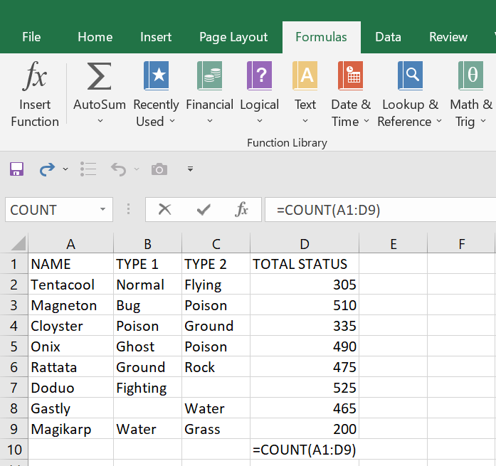
• COUNT: This function enumerates cells exclusively housing numeric values. It disregards cells containing text values, special characters, and those that are devoid of content. 

Here's a visual representation of the COUNT function in action.

‍

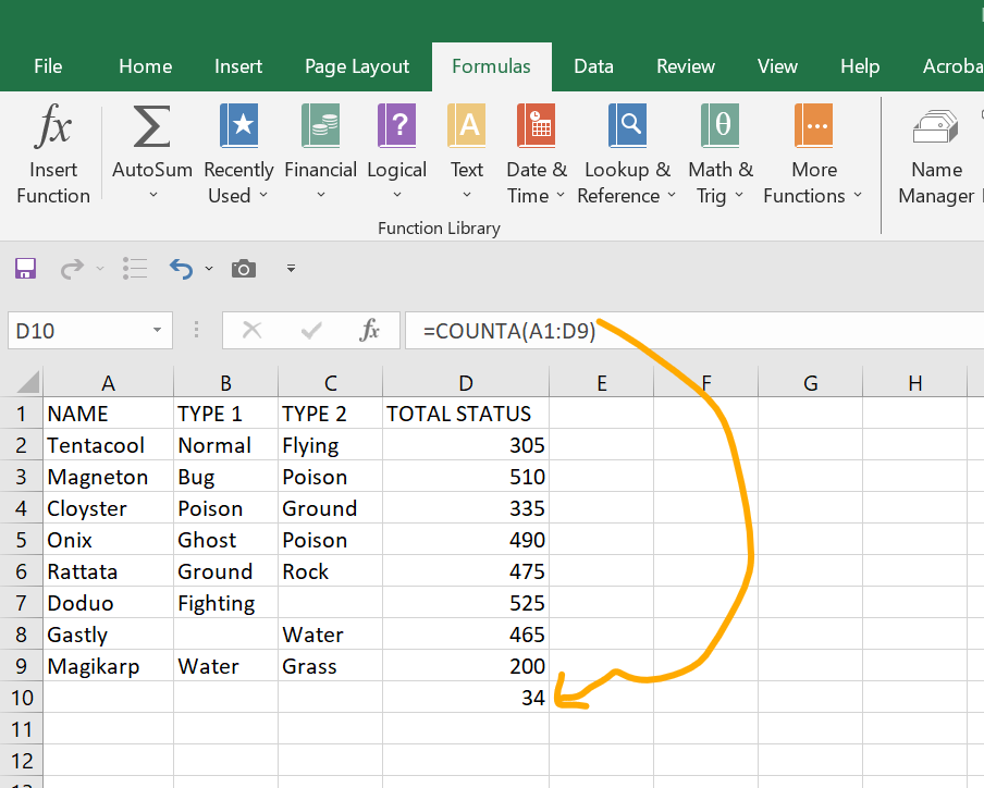
• COUNTA: Tallying every cell encompassing any form of content is the forte of COUNTA. Whether it's text values, numeric entries, or unique characters, all contribute to the count. Nevertheless, cells devoid of content are excluded from consideration. 

Here's an example showcasing the COUNTA function.

‍

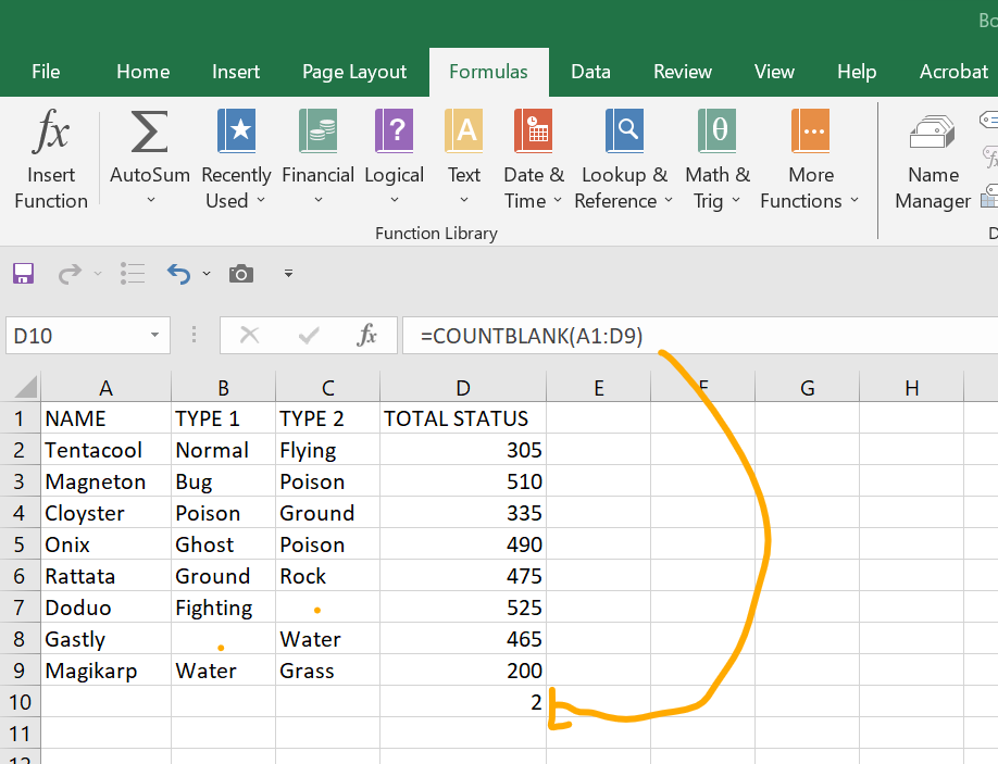
• COUNTBLANK:As the moniker implies, COUNTBLANK focuses solely on counting vacant/ empty cells. Cells laden with content don't enter the equation. 

Here's a demonstration illustrating the COUNTBLANK function.

‍

In essence, these variations of the COUNT function equip you to tailor your counting strategy according to the nature of data within your spreadsheet.

4. How to calculate compound interest in Excel? 

To compute compound interest within Excel, the Future Value (FV) function proves instrumental. FV facilitates the determination of an investment's future value, factoring in the consistent interest rate and periodic payments.

SYNTAX: FV(rate, nper, pmt, pv, type)

Deriving the rate entails dividing the annual rate by the number of periods (annual rate / periods). The count of periods (nper) emerges from the multiplication of the term's number of years by the number of periods (term * periods). The periodic payment (pmt) can assume any value, even zero. Pv and type are optional. If pmt is not mentioned, then pv should be mentioned.

5. What is the use of Timeline in Excel?

Timeline is used to filter the dates interactively by year, month, quarter and day. 

6. Explain the exact match with an example. 

For an exact match, designate the range_lookup value as FALSE or represented by 0.

EXAMPLE:

Suppose you intend to retrieve an employee's job title. Follow these steps:

• Choose the target cell and input "="
• Utilize VLOOKUP
• Define the lookup_value (in this instance, it's the ID) along with the other relevant parameters
• Set the range_lookup value to FALSE
• The function would appear as follows: =VLOOKUP(104, A1:D8, 3, FALSE)

7. What is the what-if analysis in Excel?

The What-If Analysis feature in Excel serves as a valuable forecasting tool for conducting intricate numerical computations, experimenting with data, and assessing diverse scenarios.

Consider the following example: Suppose you're posed with the question, "If you achieve $10,000 in sales over the next few months, what level of profit can you anticipate?"

• Such inquiries can be addressed effectively using the What-If Analysis feature.
• Navigate to the Data tab and click on What-If Analysis located under the Forecast section.
• The Scenario Manager proves useful for comparing multiple scenarios.
• Goal Seek facilitates reverse calculations to achieve desired outcomes.
• The Data Table is employed for sensitivity analysis.

8. How to perform HLOOKUP in Excel? 

To execute a horizontal search, you'll utilize the HLOOKUP function.

SYNTAX:

HLOOKUP(lookup_value, table_array, row_index_num, [range_lookup])

Here:

• lookup_value represents the value you wish to locate which should be located in the 1st/ top most row of the table array.
• table_array denotes the range from which data is to be extracted.
• row_index_num specifies the row containing the desired value with respect to the table array .
• [range_lookup] is a logical value, either TRUE or FALSE (TRUE or represented by 1 finds the closest match, while FALSE or represented by 0 seeks an exact match).

9. What is the “AND” function in Excel?

The Excel AND function serves the purpose of determining the truth of a singular condition or a series of conditions. If all conditions align, this function yields a TRUE boolean value.

SYNTAX:

AND(logical1, [logical2], ...)

Here,

logical1, logical2, and so forth, represent logical conditions numbered from 1 to 255 that you intend to assess.

10. How to automatically execute a macro when opening a workbook in VBA?

To automatically execute a macro when opening a workbook in VBA, candidates often suggest the following steps:

• Launch the VBA editor using the shortcut Alt+F11.
• Double-click "ThisWorkbook" on the left side of the Project Explorer.
• Insert the code "Private Sub Workbook_Open()" and press Enter.
• Insert the recorded code between "Private Sub Workbook_Open()" and "End Sub".
• After completing the code, close the VBA editor.
• SaveAs your workbook in the Excel Macro-Enabled Workbook (XLSM) format.

These steps ensure that the designated macro runs automatically upon opening the workbook. Also ensure that the Developer tab in ribbon is enabled.To do so, right click anywhere on the ribbon and choose Customize the Ribbon and check the developer tab on the right pane of the dialog box and click OK.

11. What are the 3 core modules in VBA? 

VBA encompasses three primary core modules:

• Class Modules: Class modules empower users to forge new objects and enhance existing ones. Through class modules, custom objects can be created, enhancing the versatility of VBA applications.
• User Forms: User forms constitute a module type specialized in constructing graphical user interfaces (GUIs). They play a pivotal role in designing visually interactive interfaces for applications.
• Code Modules: Typically serving as the default modules, code modules are where functions and procedures are authored. These modules form the coding backbone of VBA projects, facilitating the implementation of various functionalities.

12. What is the purpose of the Flash Fill function on Excel?

Flash Fill represents Excel functionality enabling swift data population in cells, leveraging user actions as cues. Frequently enabled by default, utilizing Flash Fill is as simple as initiating typing. When Excel detects a discernible pattern, it proactively proposes data for the respective cell. Accepting the suggested data in Flash Fill involves hitting the Enter key. In cases where Flash Fill is deactivated, reactivating it entails navigating to Tools > Options > Advanced > Editing Options, and checking the "Automatically Flash Fill" checkbox.

13. What is the SUMIF function in Excel?

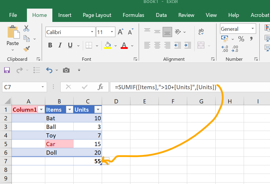
To determine the sum of data meeting specific conditions or criteria, the SUMIFS function proves useful. For instance, if you've established conditional formatting for Excel cells and seek the sum of cells exhibiting a particular format, your formula could resemble =SUMIF(range, criteria, sum_range). 

             See the example here: 

‍

14. When is the CONCATENATE function used in the Excel? 

The CONCATENATE function serves to amalgamate information from multiple cells into a singular cell. For instance, if a table contained distinct columns for first and last names, the CONCATENATE function would seamlessly merge these data points into a single column containing both the first and last name.

15. How to use SUM with the AGGREGATE function in Excel? 

We're familiar with the functioning of the SUM function, where it aggregates values and provides their total. However, in this instance, we'll employ the SUM function in the presence of error values and hidden rows. Meanwhile, here is an example of using the AGGREGATE function with option 7 to sum values while ignoring hidden rows and error values.Suppose you have the following data in Excel:

‍

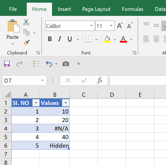
In column A, you have a list of numbers, and in column B, you have corresponding values. Cell B3 contains the #N/A error value, and cell B5 is hidden. Now, let's say you want to calculate the sum of the values in column B, but you want to ignore the error value in B3 and the hidden row in B5.

You can use the AGGREGATE function to do this: =AGGREGATE(9, 7, B2:B6). 9 represents the function number, indicating that you want to perform the SUM function.

7 is the option parameter, which specifies that you want to ignore hidden rows and error values. B2:B6 is the range of cells containing the values you want to sum. The result of this formula will be:

16. What is the CONCAT function in Excel? 

In the MS 365 version, the CONCAT function takes over the role of the CONCATENATE function. It possesses the ability to merge cell content from various ranges and/or strings. However, similar to the CONCATENATE function, it lacks the provision for specifying delimiters or using IgnoreEmpty arguments. Let's delve into the process of combining cells using the CONCAT function:

            Steps:

In the required cell, input the following formula:

=CONCAT(B5:C5)

Alternatively, type CONCAT( and select the range of cells you wish to combine, then close the parenthesis and hit the Enter key. Employ the fill handle icon to drag the formula down. Observe the resultant outcome displayed below. This function facilitates the unification of cells in Excel without the need for delimiters or handling empty cells.The sole advantage of this function compared to CONCATENATE is its capability to combine one or multiple ranges of cells. However, it lacks the provision of including a delimiter.

17. How to use the FIND function in Excel to Extract the Position of a Specified Character in a Text?

In essence, the FIND function aids in determining the position of a specified character within a given text string in Excel.

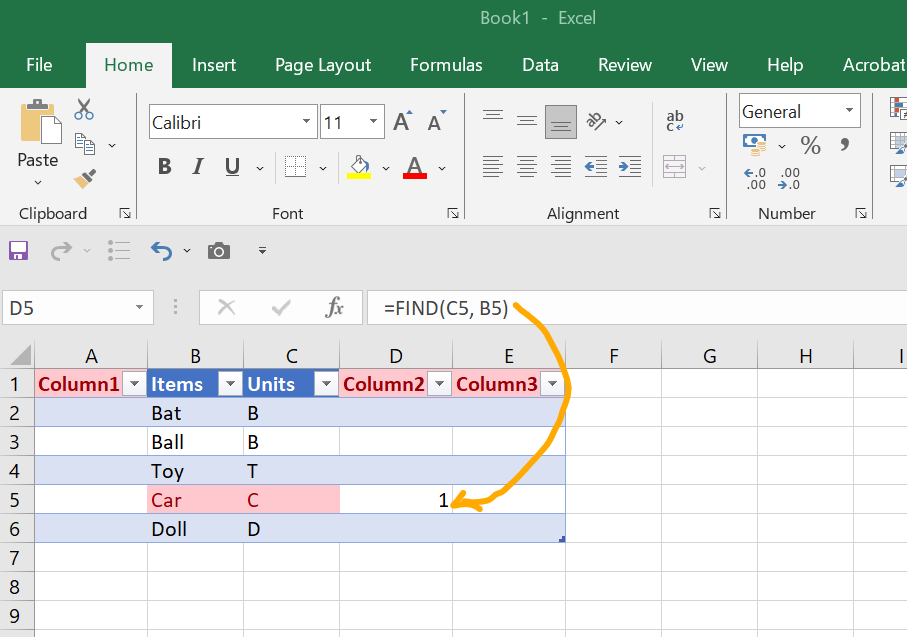
In the given illustration, Column B contains a selection of text values, while Column C outlines the specific characters to be located within the contents of Column B. Our aim in Column D is to extract the positions of the designated characters as defined in Column C.

For Cell D5, the formula employing the FIND function is as follows:

=FIND(C5, B5)

After hitting Enter, the outcome produced by the function is 2. This indicates that the letter 'a' occupies the 2nd position within the text present in Cell B5. Similar outputs can be derived for Cells D6 and D7.

Here is a sample image for better understanding.

‍

‍

18.  What is the STDEV function? 

The STDEV function is used to calculate the standard deviation of a range of cells in Excel. For example, =STDEV(A1:A10) would calculate the standard deviation of the values in cells A1 through A10.

19. What is the default value of the last parameter of the VLOOKUP function in Excel?

In case the final parameter isn't explicitly set using TRUE or FALSE, the default return value will be TRUE (approximate). This results in an approximate match being displayed for the specified query.

20. What is the main limitation of the VLOOKUP function in Excel? 

The VLOOKUP function operates unidirectionally, specifically from left to right. Consequently, the data you intend to retrieve must be positioned in a column to the right of the lookup value's location and the lookup value should be located in the first/ leftmost column of the selection/ table array.

In more recent iterations of Excel, a successor to VLOOKUP has emerged under the name XLOOKUP. Unlike its predecessor, XLOOKUP functions bidirectionally, allowing searches in any direction, and it defaults to exact matches rather than approximations. While it's anticipated that XLOOKUP will eventually supplant VLOOKUP, this transition won't take place until a significant majority of users have migrated from using older Excel versions.

21. Which is one of the most common Error messages in Excel?

One of the most prevalent error messages in Excel is the #### error. This error occurs when a cell's dimensions aren't sufficient to display the entirety of inputted data. To rectify this, simply expand the cell's width or height by dragging it accordingly. If the error still persists, then check the format of the cell and choose the appropriate format to get rid of the error.

22. How do you refresh a Pivot Table in Excel? 

To update a pivot table, you have several options:

• Click on the pivot table, go to the Analyze tab, and then choose Refresh from the pivot table tools menu.
• Right-click on the pivot table and select Refresh.
• Click on the pivot table, Utilize the keyboard shortcut Alt+F5.

For refreshing all pivot tables within a workbook simultaneously, click the arrow located beneath the Refresh button in the pivot table tools menu. Then, opt for Refresh All.

23. How to insert a drop down menu in Excel?

To establish a dropdown menu in Excel, follow these steps:

• Highlight the cells intended to host the dropdown lists.
• Navigate to the Data tab and click on Data Validation.
• A dialog box will emerge, enabling the selection of permissible inputs for these cells.
• Opt for "List" and input the dropdown menu options (separated by commas, without spaces) into the Source box.
• Click OK and the selected cells will have the dropdown as desired.

24. How do you extract a first name from a full name? 

There exist three techniques for extracting the first name from a full name. The first approach involves employing the FIND and LEFT functions. By utilizing the FIND function, you can locate the delimiter that separates the first name from the last name. Typically, this delimiter might be a space, comma, or any other symbol.

The FIND function furnishes the numeric position of this designated delimiter (with the text's initial character being assigned position 1). Subsequently, the LEFT function can be employed to extract the number of characters specified by the FIND function, starting from the text's beginning (i.e., the left side).

However, it's important to note that the value yielded by FIND includes the delimiter itself. Therefore, to pinpoint the precise endpoint of the first name, a subtraction of 1 is necessary. The resultant formula would take the form: =LEFT(A1, FIND(" ", A1) - 1).

The second method involves segregating first names and last names into distinct new columns. This is accomplished using the Text to Columns feature accessible through the Data tab. The Text to Columns dialog box facilitates the selection of the delimiter that separates each field (such as a space), while also providing a preview of the resulting split. The final step permits you to determine where the outcome should be displayed.

The third method involves inputting the first name in the first few cells in the adjacent column. Then select the entire range where the first name needs to be displayed starting from the first cell from where the sample data is filled. Using Flash fill, we can get the desired output of First names. To do so, press CTRL+E or Ribbon → Home tab → Editing section → Fill dropdown → Flash fill.

25. How Do You Clear Formatting in Excel Without Removing the Cell Content?

Highlight the cells from which you want to eliminate all formatting, then navigate to the Home tab. Within the Editing section of the tab, access the dropdown menu by clicking on the Clear button. Choose Clear Formats. Alternatively, you can use the keyboard shortcut Alt+E+A+F or alternatively Alt+H+E+F.

Conclusion 

It's a wise approach to adequately prepare yourself for any interview, ideally well in advance, allowing ample time to address any gaps in your knowledge, CV, or portfolio. To assess your level of readiness, you can refer to the following checklist of advanced level questions and answers for Excel interviews.

Advanced Excel Questions and answers serve as a valuable tool for gauging and refining one's aptitude in data management and analysis through Excel. These Advanced Excel questions and answers play a pivotal role in pinpointing areas of enhancement for both individuals and organizations, simplifying the attainment of their data management and analytical objectives. Also, you can get upskilled in Excel Efficiency course at keySkillset.

‍