What is Conditional Formatting?

Conditional formatting in Excel is a feature in many spreadsheet applications that allows you to apply specific formatting to cells that meet certain criteria. It is most often used as color-based formatting to highlight, emphasize, or differentiate among data and information stored in a spreadsheet.

Conditional formatting enables spreadsheet users to do a number of things. First and foremost, it calls attention to important data points such as deadlines, at-risk tasks, or budget items. It can also make large data sets more digestible by breaking up the wall of numbers with a visual organizational component. Finally, conditional formatting can transform your spreadsheet (that previously only stored data) into a dependable “alert” system that highlights key information and keeps you on top of your workload.

^{Conditional Formatting Basics}

Before we walk you through creating and applying conditional formatting in Excel, you should understand the basics. The following structural aspects of Excel conditional formatting will guide how you create and apply rules:

If-Then Logic

All conditional formatting rules are based on simple if-then logic: if X criteria are true, then Y formatting will be applied (this is often written as p → q, or if p is true, then apply q). You won’t have to hard-code any logic, though – Excel and other spreadsheet apps have built-in parameters so you can simply select the conditions you want the rules to meet. Advanced users can also apply the program’s built-in formulas to logic rules.

Preset Conditions

Excel has a huge library of preset rules encompassing nearly all functions that beginner users will want to apply. We will familiarize you with several of the most popular ones in the next section.

Custom Conditions

For situations where you want to manipulate a preset condition, you can create your own rules. If appropriate, you can use Excel formulas in the rules you write.

Applying Multiple Conditions

You can apply multiple rules to a single cell or range of cells. However, be aware of rule hierarchy and precedence – we will show you how to manage stacked rules in the walk-through.

Overall, applying conditional formatting is an easy way to keep you and your team members up to date with your data. For example: calling visual attention to important dates and deadlines, tasks and assignments, budget constraints, and anything else you might want to highlight. When applied correctly, conditional formatting will make you more productive by reducing the time spent manually, combining data and making it easier to identify trends, so you can focus on the big decisions.

Conditional Formatting of the Data Table

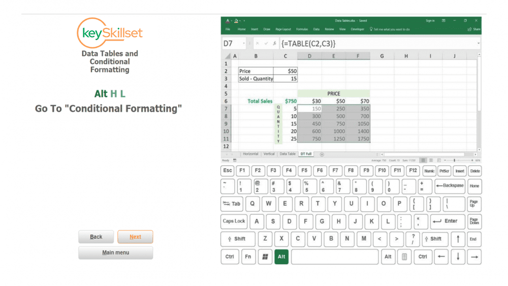
Let’s apply conditional formatting to our data tables we have created in the previous blog (LINK). For that, you need to highlight the gist of the data table (D7 – F11). Then go to “Conditional Formatting” using the shortcut Alt H L clicking one after another (Alt to access the Ribbon, H for Home, L for Conditional Formatting).

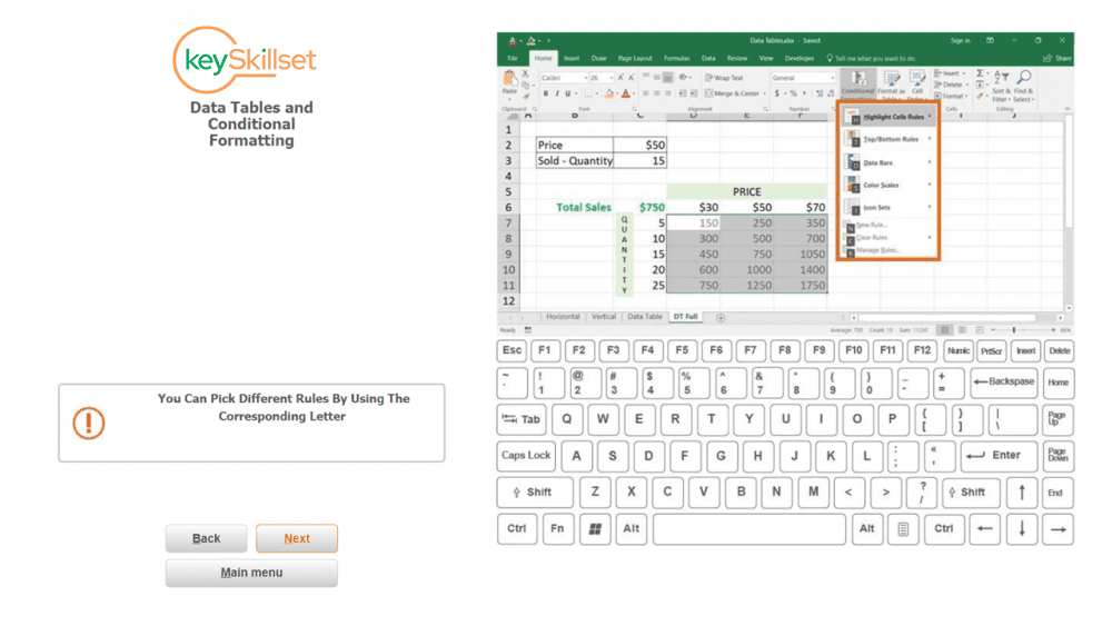
In the menu appeared, you can pick different rules for conditional formatting using the corresponding letter.

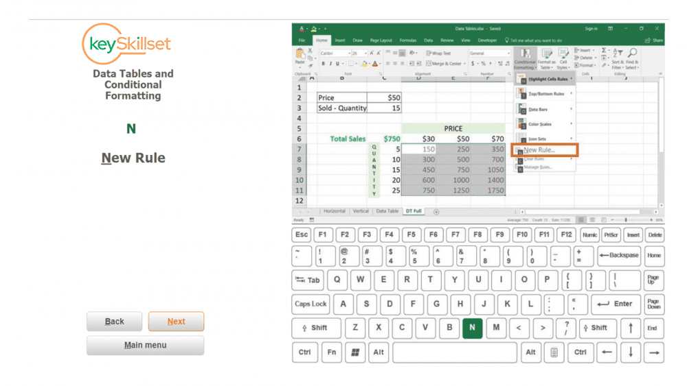
Let’s say we’d like to create a new rule, so let’s click N for that.

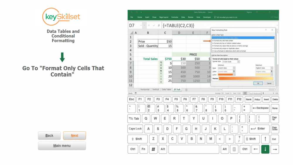
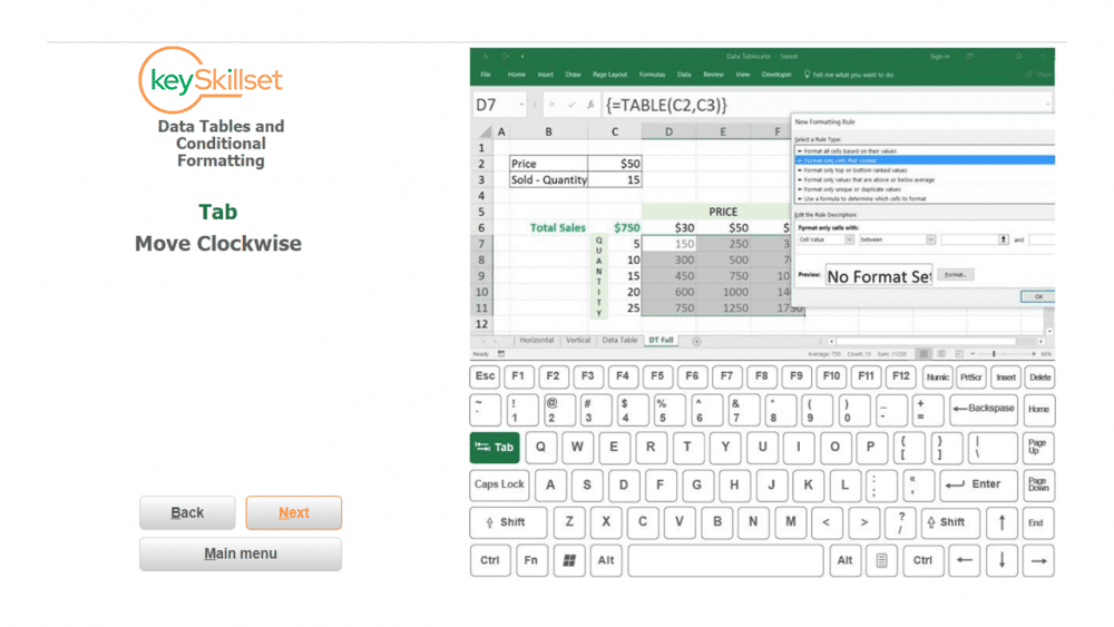
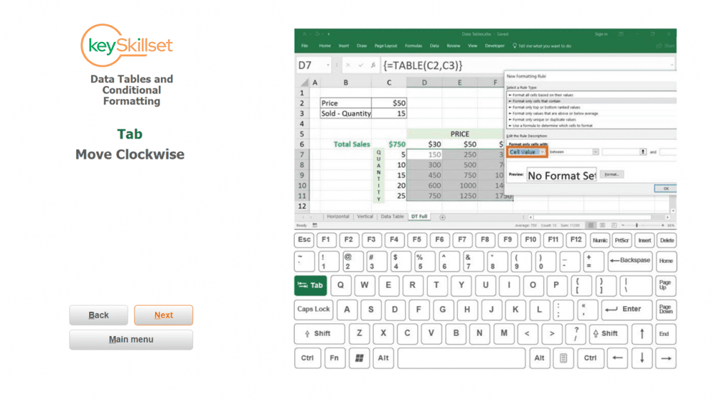
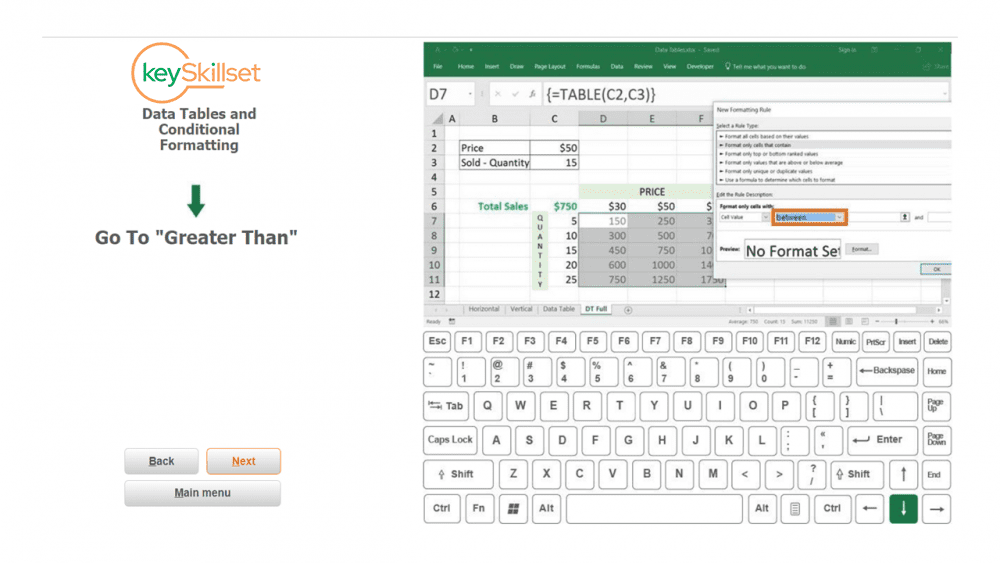
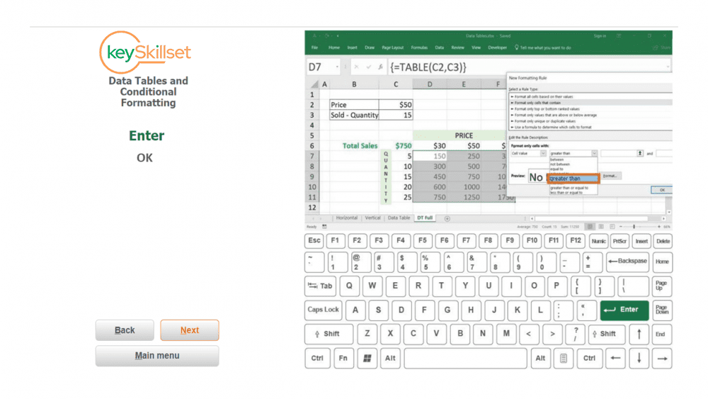
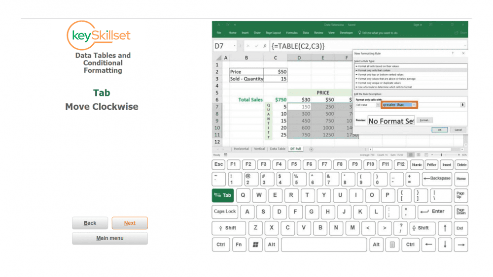
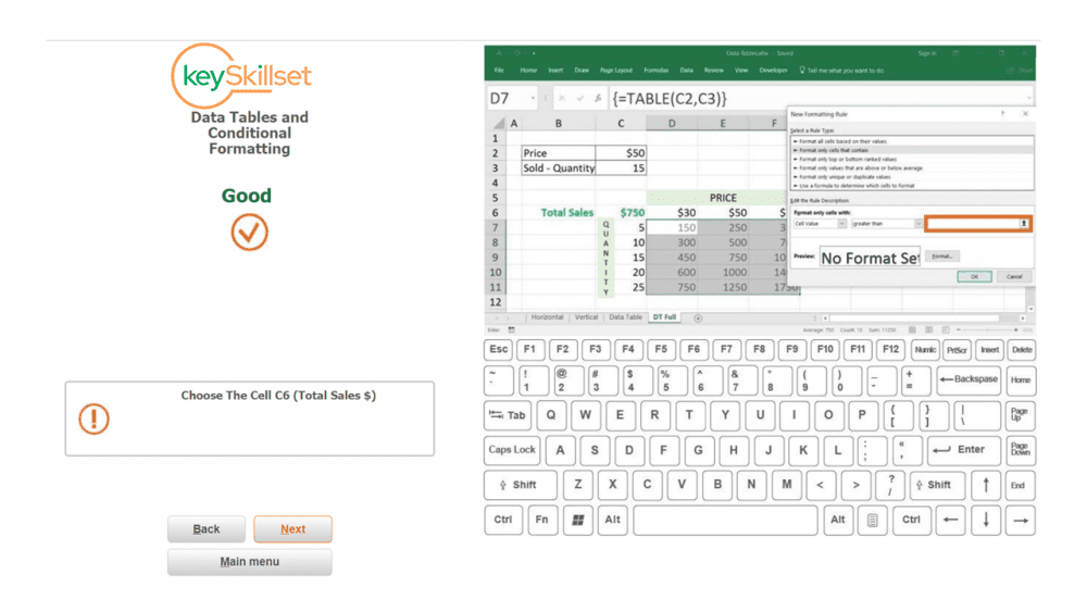
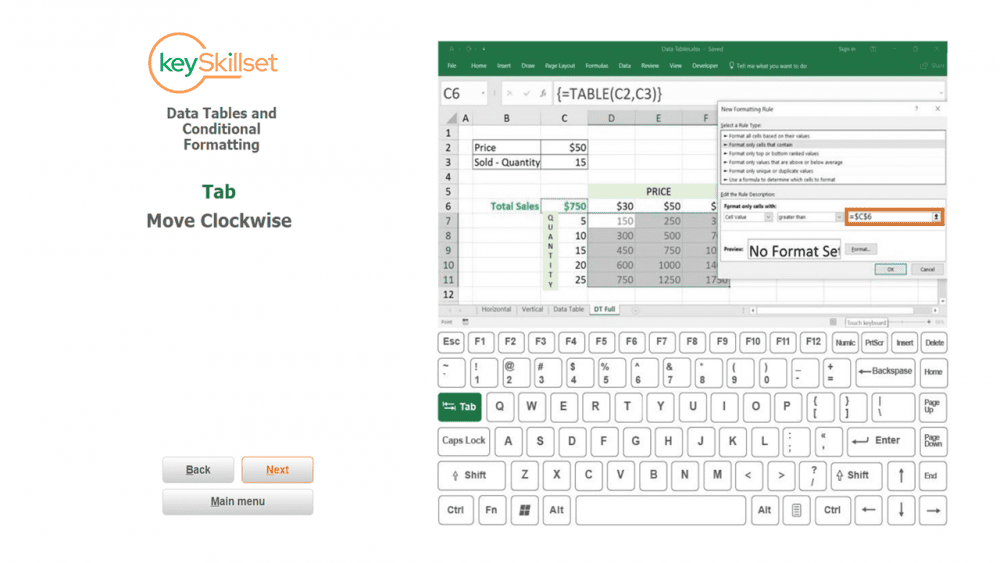
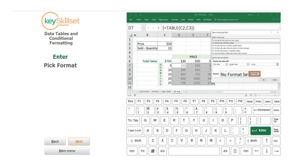
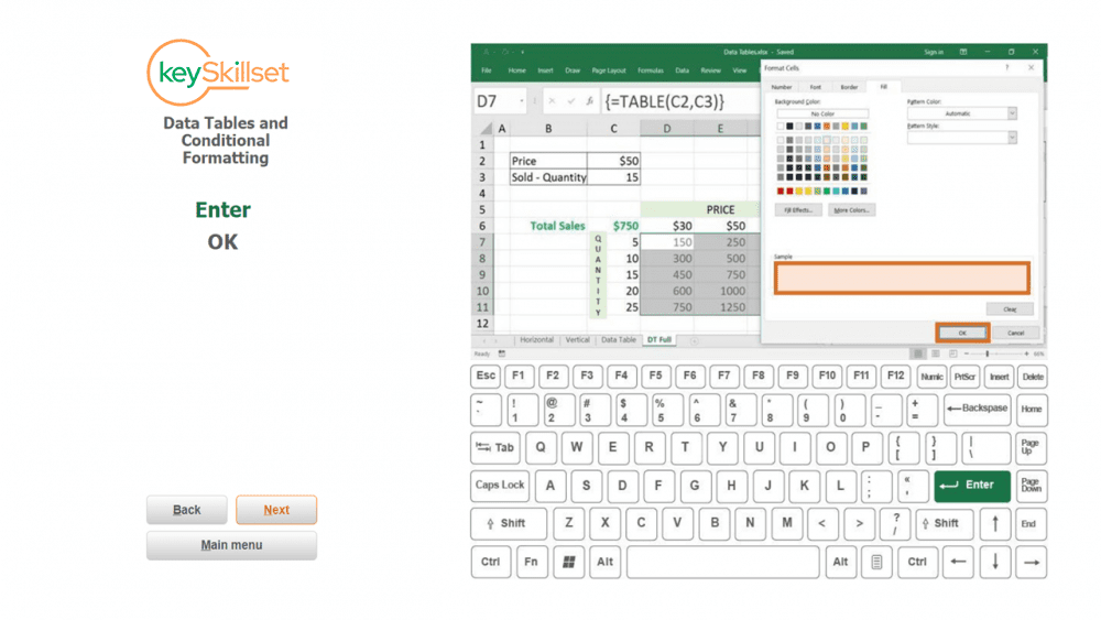
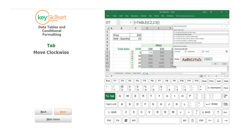
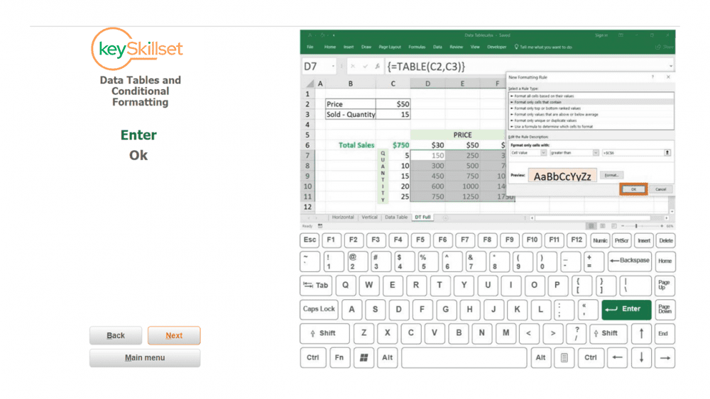
In our example, we want to put in a different color the cells in the data table that contain values greater than $750 (Total Sales, cell C6). Follow the logic of the screenshots below to understand how to make it happen.

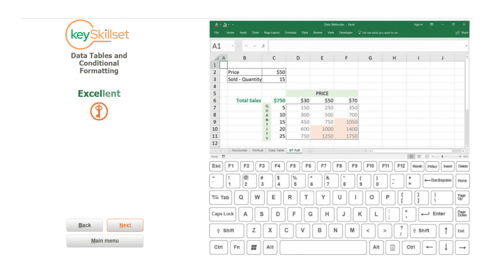
Great job! On the last screen, above you can see that we put the data table cells in color if the value is greater than $750. Mission accomplished!

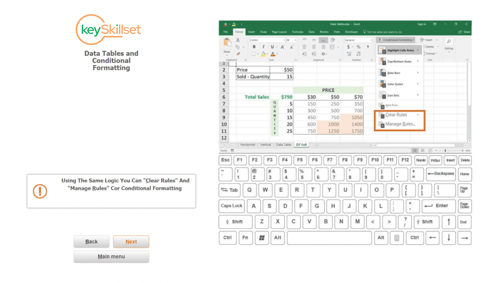
Using the same logic, you can “Clear Rules” that you have created before (shortcut would be Alt H L C). Otherwise, use “Manage Rules” if you’d like to change something in the conditional formatting rules you have created (shortcut would be Alt H L R).

Conclusion

Conditional formatting provides visual cues to help you quickly make sense of your data. Every Excel trick you learn makes you one step closer to being proficient and quick in Excel. Moreover, you can spend less time on the spreadsheets and more on the things you love doing. Follow our blogs and play keySkillset Game to be hundreds of steps closer to that.

‍